Tullock Lottery Contests with Direct and Covert Discrimination

Matthew W. Thomas Tullock Lottery Contests with Direct and Covert Discrimination Thursday. April 15, 2021

These notes summarize concepts introduced in Nti (1999), Fang (2002), Nti (2004), Epstein et al (2013), and Ewerhart (2017a) about revenue maximization in Tullock lottery contests.

Introduction

Contests are models of conflict where risk neutral players exert costly effort to win a prize. A lottery contest is any contest where there is not a deterministic relationship between effort and victory. For example, scores could be measured incorrectly or there could be some randomness in the relationship between effort and the final scores. Alternatively, you can interpret lottery contests as giving each player a slice of a prize. For example, a 5% probability of receiving the prize is the same as receiving 5% of the prize with certainty.

The most popular lottery contest is the Tullock contest.^[1] We discuss ways to increase competitiveness in Tullock contests by discriminating against the stronger player. Handicaps in sporting events are a real world example of such discrimination. The purpose of a handicap is to make a match more even so that both teams/players exert more effort.

Model

Suppose that the prize of contest is worth one to both players. So, the two players have the same value. However, their scores have different costs. In particular, we will say that the score is $k > 1$ times more costly for Player 2 than for Player 1.^[2] You can interpret this as saying that Player 1 is more skilled. So, it takes less effort for her to produce a high score.

The probability of Player 1 winning the prize in a Tullock contest when she chooses score $s_1$ and her opponent chooses score $s_2$ is:

$$p_1(s_1, s_2) = \frac{s_1^{r}}{s_1^{r} + (\delta s_2)^{r} }.$$

The parameter $\delta$ sets the level (and direction) of direct discrimination. If $\delta = 0$$, then Player 1 always wins. If $\delta = \infty$$, then Player 2 always wins. In general, $\delta > 1$ implies discrimination against Player 1. Note that the prize is symmetric when $\delta = 1$. In this case, there is no direct discrimination.

The other parameter, $r$, is more subtle. It affects the variance of the lottery in the contest. If $r \to \infty$, the prize always goes to the player with the higher score.^[3] If $r = 0$, the prize is allocated at random. This precision parameter changes the marginal returns to effort at different levels. For example, if $r < 1$, then the lower effort player gets a disproportionately high return. While such a contest is fair, in the sense that the two players are not treated differently, it is actually rigged in favor of the weaker player.

The final payoffs are:

$$U_1(s_1, s_2) = \frac{s_1^{r}}{s_1^{r} + (\delta s_2)^{r} } - s_1$$

$$U_2(s_1, s_2) = \frac{(\delta s_2)^{r}}{s_1^{r} + (\delta s_2)^{r} } - k s_2$$

Assumptions

We consider pairs $r, \delta$ such that the following two conditions are satisfied.

1. No reversal: $\delta \leq k$
2. Pure strategy equilibrium: $\left( \frac{\delta}{k} \right)^{r} \geq r - 1$

The first assumption prevents excessive discrimination against Player 1 and is without loss of optimality. This is made for simplicity. Without it, we would have to consider more cases.

The second assumption is more important. It is a necessary and sufficient condition for there to be an equilibrium in pure strategies. It is always satisfied if $r \leq 1$ and is never satisfied if $r > 2$. The condition is equivalent to

$$r \leq \bar{r}(\delta/k) = 1 - \frac{W \left( - (\delta/k) \log{\left( \delta/k \right)} \right)}{\log{\left( \delta/k \right)}}$$

where $W$ is the Lambert W function. The upper bound, $\bar{r}$ is a strictly increasing function.

It is not obvious, but this condition is also without loss of optimality.

Equilibrium

To find the Nash equilibrium, we need to find the best response functions for each of the players. We do this by maximizing each payoff function. Player 1’s first order condition is

$$\frac{r s_1^{r} (\delta s_2)^{r}}{s_1 \left(s_1^{r}+(\delta s_2)^{r}\right)^2} = 1$$

and Player 2’s first order condition is

$$\frac{r s_1^{r } (\delta s_2)^{r}}{s_2 \left(s_1^{r}+(\delta s_2)^{r}\right)^2} = k.$$

This is a system of two equations with two unknowns. Dividing the second by the first gives us $k = \frac{s_1^{\star}}{s_2^{\star}}$. So the ratio of the scores does not depend on the discrimination parameters. Thus, any change that increases one also increases the other. With this, we can quickly solve the system of equations to get $s_1^{\star} = \frac{r (k \delta)^{r} }{\left( k^{r}+\delta^{r} \right)^2}$ and $s_2^{\star} = \frac{r (k \delta)^{r} }{k \left( k^{r}+\delta^{r} \right)^2}$.

In order for the first order approach to be valid, we have to check the second order and boundary conditions.

The second order conditions require the second derivative of the payoffs to be negative at the equilibrium. They are satisfied if and only if $\left( \frac{k}{\delta} \right)^{r} > \frac{r - 1}{r + 1}$. This inequality holds by Assumption 1.

The boundary conditions require that payoffs are non-negative at the proposed equilibrium. Otherwise, the player would prefer to chose a score of zero. Using $k = \frac{s_1^{\star}}{s_2^{\star}}$, we can dramatically simplify the equilibrium payoffs:

$$U_1(s_1^{\star}, s_2^{\star}) = \frac{k^{r}}{k^{r} + \delta^{r}} - s_1^{\star}$$

$$U_2(s_1^{\star}, s_2^{\star}) = \frac{\delta^{r}}{k^{r} + \delta^{r}} - s_1^{\star}.$$

By Assumption 1, $U_2(s_1^{\star}, s_2^{\star}) \leq U_1(s_1^{\star}, s_2^{\star})$. So, we only need a condition such that Player 2 has a positive payoff. Substituting $s_1^{\star} = \frac{r (k \delta)^{r} }{\left( k^{r}+\delta^{r} \right)^2}$ gives our lowest payoff

$$U_2(s_1^{\star}, s_2^{\star}) = \frac{\delta^{r}}{k^{r} + \delta^{r}} - \frac{r (k \delta)^{r} }{\left( k^{r}+\delta^{r} \right)^2}.$$

It’s not obvious that this is non-negative by Assumption 2. However, it just requires some factoring.

Contest design

Suppose that there is some contest designer who can choose $r$ and/or $\delta$ in order to maximize the revenue, $s_1 + s_2$. Because we know that $k = \frac{s_1}{s_2}$, we are actually trying to maximize $(1 + k^{-1}) s_1$. Because $k$ is constant, maximizing $s_1$ is enough.

Direct discrimination

Suppose $r$ is fixed. For now, assume it is one. To maximize revenue, we need to maximize $s_1$. Suppose that we can directly discriminate using $\delta$. Then, our problem is

$$\max_{\delta} \frac{k \delta}{( k + \delta )^2}.$$

This maximum is obtained at $\delta^\star = k$.

In this case, the revenue is

$$\begin{aligned} s_1 + s_2 &= \left( 1 + \frac{1}{k} \right) s_1 \\ &= \left( 1 + \frac{1}{k} \right) \frac{k^2}{( 2 k )^2} \\ &= \frac{1 + k}{4 k} \end{aligned}$$

If we allow $r$ to take any positive value, then the optimal delta will still be $\delta^\star = k$. This result comes from the optimization problem

$$\max_{\delta} \frac{r (k \delta)^{r} }{\left( k^{r}+\delta^{r} \right)^2}$$

which has the following first order condition:

$$\frac{r^2 ( \delta k)^{r} ( k^{r} - \delta^{r} )}{ \delta ( k^{r} + \delta^{r} )^3 } = 0.$$

Covert discrimination

Suppose that the contest designer cannot discriminate directly. So $\delta = 1$, and the designer chooses $r$ in order to maximize the revenue of the contest. Then, our problem is

$$\max_{r} \frac{r k^{r}}{( 1 + k^r )^2}.$$

If we take first order conditions and solve, we get

$$r = \frac{1}{\log(k)} \left( 1 - \frac{2}{1 + k^{r}} \right)^{-1}$$

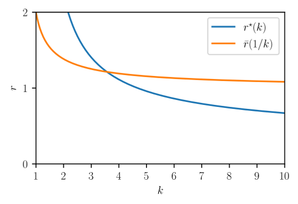
which defines implicit function $r^\star(k)$. However, these values cannot be attained unless $k$ is sufficiently large. Recall that there is no pure strategy equilibrium if $r > \bar{r}$. So, there is no way to reach some of these values.

If you set up a Lagrangian as in Proposition 3 of Nti (2004), then you find that the constrained optimum is the minimum of the two pictured curves. No exact representation of the intersection is known. However, it is approximately $k = 3.509$.

Overall optimum

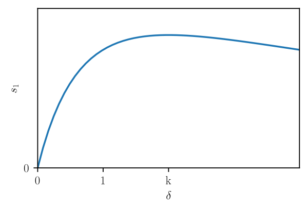
We know that if both forms of discrimination are allowed, then $\delta^\star = k$ because this is the optimum for any $r$. As you can see in the first plot, this means that $\bar{r} = 2$. We will show that this is also the constrained optimum. Our optimization problem is

$$\max_{r \leq 2} \frac{r}{4}$$

which is obviously attained at $r = 2$. So, the optimal revenue is $(1 + k^{-1}) \frac{2}{4} = \frac{1 + k}{2 k}$.

Beyond pure strategies

Assumption 2, which guarantees that equilibria exist in pure strategies is without loss of optimality. So, the solutions in the previous sections hold for all $r \geq 1$.

If payoffs are symmetric, Assumption 2 is violated if and only if $r > 2$. In this case, Baye et al. (1994) shows that when there is a symmetric mixed strategy equilibrium in which both players receive a payoff of zero.^[4] This means that when $\delta = k$,

$$\begin{aligned} E[s_1] &= E \left[ \frac{s_1^{r}}{s_1^{r} + (k s_2)^{r} } \right] \\ k E[s_2] &= E \left[ \frac{(k s_2)^{r}}{s_1^{r} + (k s_2)^{r} } \right] \end{aligned}$$

Symmetry implies that that each player’s expected probability of winning is one half. Therefore, $E[s_1] = \frac{1}{2}$, $E[s_2] = \frac{1}{2 k}$, and $E[s_1 + s_2] = \frac{1 + k}{2 k}$. This is the same maximum revenue as in the overall optimum in pure strategies. It’s not obvious that this is the maximum revenue. For example, one might imagine that the principal could ensure zero payoffs but have Player 1 win with probability greater than one half. In order to confirm that Assumption 2 is without loss of optimality, we need to answer a few questions.

Are equilibria revenue equivalent? Yes. Ewerhart (2017a) shows that the equilibrium is unique when $r \leq 2$ and Ewerhart (2017b) shows that equilibria are revenue and payoff equivalent when $r > 2$.

Is $r \in (\bar{r}( \delta / k ), 2]$ ever optimal No. Wang (2010) shows that revenue is

$\frac{2 \delta}{r k} \left( \frac{1 + k}{2 k} \right) (r - 1)^{(r - 1)/r}$

on this interval which is weakly decreasing in $r$. Therefore, $r = \bar{r}( \delta / k )$ yields weakly greater revenue.

Is $r > 2$ ever optimal? No. Alcade and Dahm (2010) show that if $r > 2$, the Tullock contest is revenue and payoff equivalent to an all-pay auction. Revenue in this auction is $\left( \frac{\delta}{k} \right) \frac{1 + k}{2 k}$. This is the same revenue as when $r = 2$.

Is $\delta < k$ ever optimal? No. Note that the revenue in the last two points is increasing in $\delta$.

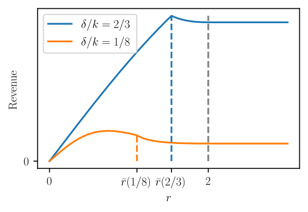
The above shows an example of how revenue depends on $r$. Note that the maximum is reached before $\bar{r}(\delta / k)$ when the players are very heterogeneous (orange) and at the upper bound when players are more homogeneous (blue).^[5]

Conclusion

This table summarizes the results that we have about each type of optimal contest. There is not much to summarize for covert discrimination because there aren’t any closed form expressions.

	$$r,\delta$$	Payoffs	Revenue
No discrimination	1, 1	$\frac{k^2}{(1+k)^2}, \frac{1}{(1+k)^2}$	$\frac{1}{k+1}$
Direct ($$r$ fixed)	$r,k$	$\frac{2-r}{4}, \frac{2-r}{4}$	$\frac{1+k}{4k}$
Covert ($$\delta = 1$$)	$r(k),1$
Unrestricted	$2,k$	0, 0	$\frac{1+k}{2k}$

The case of covert discrimination demonstrates an important precision tradeoff. Choosing a large value of $r$ increases competitiveness by awarding the prize more frequently to the player with the higher score. However, choosing a low value allows you to discriminate against the stronger player – which also increases competitiveness. The effect that wins out depends on the size of the asymmetry between players. When $k$ is large enough, this discrimination effect wins out. However, when direct discrimination is possible, there is no advantage to covert discrimination.

---

---

1. Tullock contests were introduced 1980 by Gordon Tullock. The other major lottery contest is the rank order contest (Lazear and Rosen 1981). ↩︎

2. The papers mentioned give different prize values instead of different costs. The two are equivalent. I prefer to say that one player is more skilled than to say that one player values the prize more. ↩︎

3. In this case, it is not a lottery contest. It converges to the all-pay auction – the main deterministic contest. ↩︎

4. The symmetric equilibrium is characterized in Ewerhart (2015). ↩︎

5. More figures like the above can be found in Chowdhury et al. (2020). ↩︎

---